Co-expression

1.Pipeline

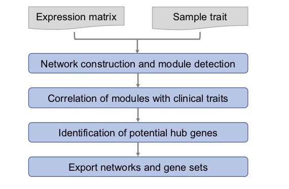
首先计算基因之间的相关系数，构建基因网络(correlation network of genes)，然后将具有相似表达模式的基因划分成模块(module)。随后计算各个模块与样本表型数据之间的相关性，对特定的感兴趣的模块分析核心基因(hub gene，通常是转录因子等关键的调控因子)，并将特定模块的基因提取出来，进行GO/KEGG等分析。

2.Data structure

2.1.Getting software & data

2.2.Input data

输入数据的准备：这里主要是表达矩阵，如果是转录组数据，最好是RPKM值或者其它归一化好的表达量。然后就是临床信息或者其它表型，总之就是样本的属性。

File name	Description
input_fpkm_matrix.rds	GSE48213 breast cancer gene expression matrix (top 5,000)
data_traits.rds	56 cell lines information for the GSM data in GSE48213

Import data

setwd("/Share2/home/lulab/xixiaochen/training_share2/co_expression/")
datExpr <- readRDS(file="/Share2/home/lulab/xixiaochen/training_share2/co_expression/input_fpkm_matrix.rds")
datTraits <- readRDS(file="/Share2/home/lulab/xixiaochen/training_share2/co_expression/data_traits.rds")

Data character

datExpr[1:4,1:4]
dim(datExpr)

#           ENSG00000210082 ENSG00000198712 ENSG00000198804 ENSG00000210845
#GSM1172844        78053.20       103151.73       112917.53        92808.32
#GSM1172845        96200.86       157203.85       163847.92        93501.17
#GSM1172846        18259.11        40704.97        13357.02        75183.17
#GSM1172847        33184.15        43673.63        15360.50        91278.61
#GSM1172848        35255.48        55018.26        17715.40        65460.84
#### each row represents a cell line (sample), each column represents the fpkm value of a gene

#[1]   56 5000
#### 56 cell lines (samples), 5000 genes

datTraits[1:4,]
dim(datTraits)

#                  gsm cellline       subtype
#GSM1172844 GSM1172844    184A1 Non-malignant
#GSM1172845 GSM1172845    184B5 Non-malignant
#GSM1172846 GSM1172846    21MT1         Basal
#GSM1172847 GSM1172847    21MT2         Basal
#### each row represents a cell line (sample), each column provides the gsm number, the cell line name and the cell line subtype information

#[1] 56  3
#### 56 cell lines (samples)
#### The rownames of datExpr and datTraits are matched.

2.3 Output data

File name	Description
FPKM-TOM-block.1.Rdata	Standarded R file contains the consensus topological overlaps for WGCNA results of the GSE48213 data
CytoscapeInput-edges-brown.txt/CytoscapeInput-edges-filter-brown.txt	Input file contains network edge information for Cytoscape
CytoscapeInput-nodes-brown.txt/CytoscapeInput-nodes-filter-brown.txt	Input file contains network node information for Cytoscape
geneID_brown.txt	Total gene ID list in specific modules

3.Running steps

WGCNA分析

基本概念

WGCNA译为加权基因共表达网络分析。该分析方法旨在寻找协同表达的基因模块(module)，并探索基因网络与关注的表型之间的关联关系，以及网络中的核心基因。

适用于复杂的数据模式，推荐5组(或者15个样品)以上的数据。一般可应用的研究方向有：不同器官或组织类型发育调控、同一组织不同发育调控、非生物胁迫不同时间点应答、病原菌侵染后不同时间点应答。

基本原理

从方法上来讲，WGCNA分为表达量聚类分析和表型关联两部分，主要包括基因之间相关系数计算、基因模块的确定、共表达网络、模块与性状关联四个步骤。

第一步计算任意两个基因之间的相关系数（Person Coefficient）。为了衡量两个基因是否具有相似表达模式，一般需要设置阈值来筛选，高于阈值的则认为是相似的。但是这样如果将阈值设为0.8，那么很难说明0.8和0.79两个是有显著差别的。因此，WGCNA分析时采用相关系数加权值，即对基因相关系数取N次幂，使得网络中的基因之间的连接服从无尺度网络分布(scale-freenetworks) ，这种算法更具生物学意义。

无尺度网络分布：大部分节点只和很少节点连接，而有极少的节点与非常多的节点连接，生物体选择scale-free network可以保证少数关键基因执行着主要功能，只要保证hub的完整性，整个生命体系的基本活动在一定刺激影响下将不会受到太大影响。

第三步得到模块之后可以做很多下游分析：（1）模块的功能富集（2）模块与性状之间的相关性（3）模块与样本间的相关系数（4）找到模块的核心基因（5）利用关系预测基因功能

3.0 Install packages

source("https://bioconductor.org/biocLite.R")
biocLite(c("AnnotationDbi", "impute","GO.db", "preprocessCore", "multtest"))
install.packages(c("WGCNA", "stringr", "reshape2"))

3.1 Library the WGCNA package

library(WGCNA)

3.2 Pick the soft thresholding power

options(stringsAsFactors = FALSE)
#open multithreading 
enableWGCNAThreads()

powers = c(c(1:10), seq(from=12, to=20, by=2))
#Call the network topology analysis function，choose a soft-threshold to fit a scale-free topology to the network
sft=pickSoftThreshold(datExpr, powerVector = powers, verbose = 5)

#pickSoftThreshold: will use block size 5000.
# pickSoftThreshold: calculating connectivity for given powers...
#   ..working on genes 1 through 5000 of 5000
#   Power SFT.R.sq  slope truncated.R.sq  mean.k. median.k.  max.k.
#1      1   0.0944 -0.904          0.885 1040.000  1.02e+03 1810.00
#2      2   0.4910 -1.580          0.952  328.000  3.03e+02  866.00
#3      3   0.7030 -1.860          0.983  128.000  1.08e+02  474.00
#4      4   0.7920 -2.000          0.991   57.300  4.38e+01  283.00
#5      5   0.8490 -2.060          0.996   28.400  1.95e+01  179.00
#6      6   0.8810 -2.090          0.991   15.200  9.45e+00  118.00
#7      7   0.9040 -2.070          0.990    8.640  4.89e+00   80.60
#8      8   0.9220 -2.040          0.994    5.170  2.67e+00   56.40
#9      9   0.9330 -2.030          0.995    3.240  1.54e+00   40.50
#10    10   0.9350 -2.020          0.989    2.100  9.29e-01   30.00
#11    12   0.9250 -2.030          0.977    0.971  3.63e-01   17.30
#12    14   0.9210 -2.020          0.982    0.496  1.56e-01   10.50
#13    16   0.9250 -1.970          0.992    0.275  7.04e-02    6.61
#14    18   0.8940 -1.960          0.973    0.163  3.31e-02    4.31
#15    20   0.9220 -1.820          0.986    0.102  1.63e-02    2.89

pdf(file="/Share2/home/lulab/xixiaochen/training_share2/co_expression/soft_thresholding.pdf",width=9, height=5)
#Plot the results:
par(mfrow = c(1,2))
cex1 = 0.9
# Scale-free topology fit index as a function of the soft-thresholding power
plot(sft$fitIndices[,1], -sign(sft$fitIndices[,3])*sft$fitIndices[,2],
     xlab="Soft Threshold (power)",ylab="Scale Free Topology Model Fit,signed R^2",type="n",
     main = paste("Scale independence"));
text(sft$fitIndices[,1], -sign(sft$fitIndices[,3])*sft$fitIndices[,2],
     labels=powers,cex=cex1,col="red");
#Red line corresponds to using an R^2 cut-off
abline(h=0.90,col="red")
#Mean connectivity as a function of the soft-thresholding power
plot(sft$fitIndices[,1], sft$fitIndices[,5],
     xlab="Soft Threshold (power)",ylab="Mean Connectivity", type="n",
     main = paste("Mean connectivity"))
text(sft$fitIndices[,1], sft$fitIndices[,5], labels=powers, cex=cex1,col="red")
dev.off()

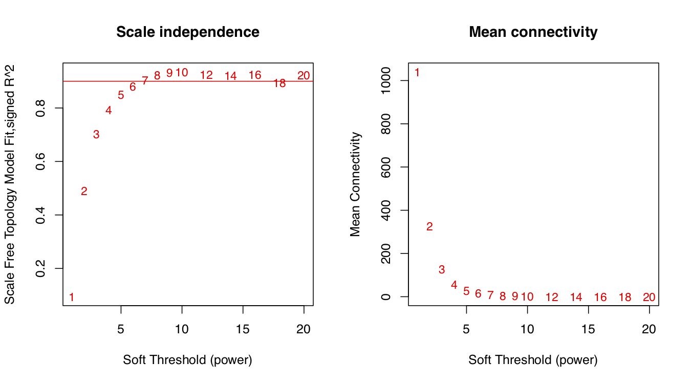
软阈值（即权重参数，可以理解为相关系数的β次幂）取值默认为1到30，上述图形的横轴均代表软阈值，左图的纵轴数值越大，说明该网络越逼近无尺度网络，右图的纵轴表示对应的基因模块中所有基因邻接性的均值。

sft$powerEstimate
#[1] 6
#best_beta = sft$powerEstimate

3.3 One-step network construction and module detection

把输入的表达矩阵的几千个基因归类成了几十个模块。大体思路：计算基因间的邻接性，根据邻接性计算基因间的相似性，然后推出基因间的相异性系数，并据此得到基因间的系统聚类树。

net = blockwiseModules(datExpr,
                 power = sft$powerEstimate,
                 maxBlockSize = 6000,
                 TOMType = "unsigned", minModuleSize = 30,
                 reassignThreshold = 0, mergeCutHeight = 0.25,
                 numericLabels = TRUE, pamRespectsDendro = FALSE,
                 saveTOMs = TRUE,
                 saveTOMFileBase = "FPKM-TOM",
                 verbose = 3)

table(net$colors)
#   0    1    2    3    4    5    6    7    8    9   10   11   12   13   14   15 
# 246 1671  355  305  279  270  241  175  168  124  108  101   88   87   84   84 
#  16   17   18   19   20   21   22   23   24   25   26   27 
#  77   67   62   61   60   47   44   41   40   40   38   37
#### table(net$colors) show the total modules and genes in each modules. The '0' means genes do not belong to any module.

3.4 Module visualization

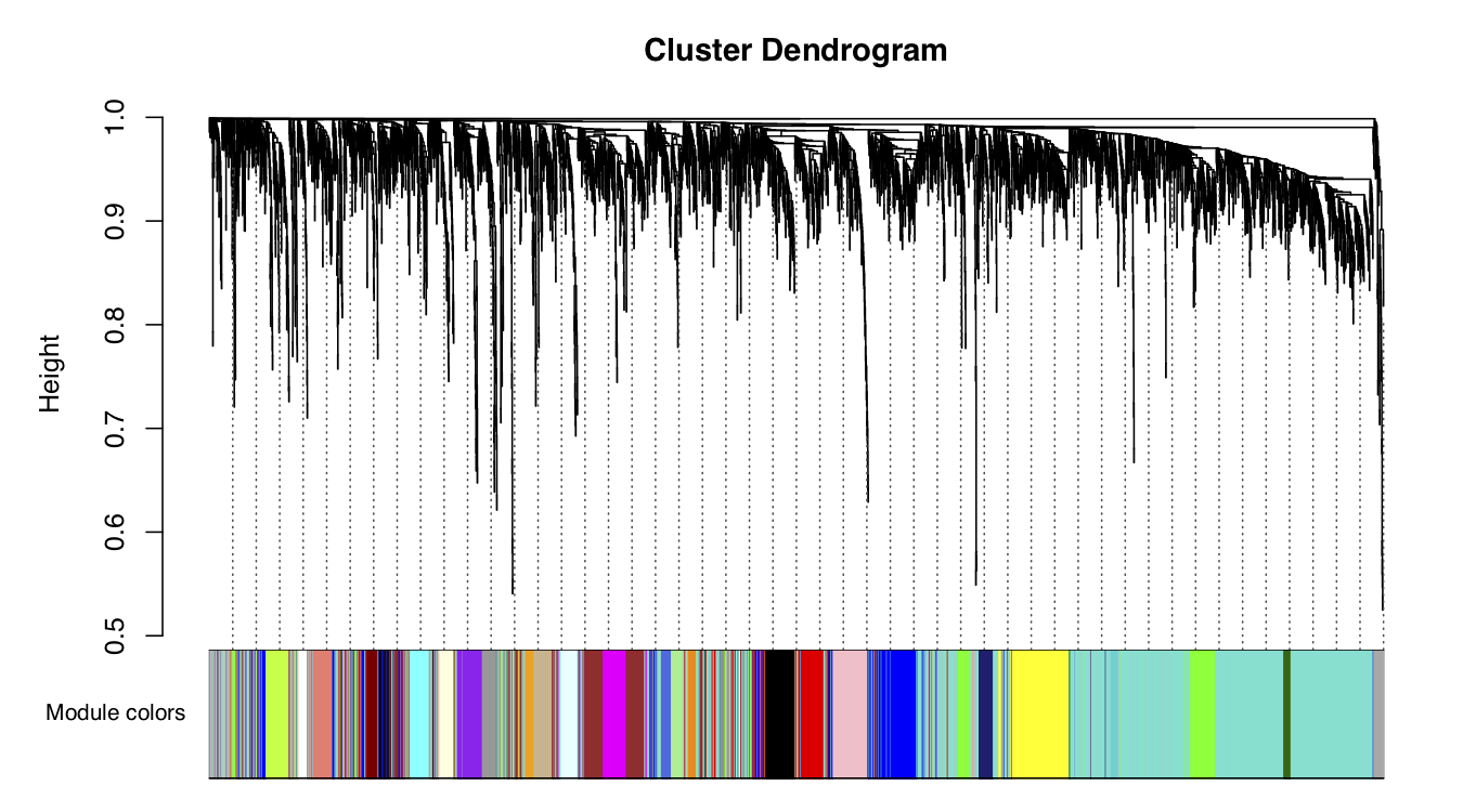
这里用不同的颜色来代表那些所有的模块，其中灰色默认是无法归类于任何模块的那些基因，如果灰色模块里面的基因太多，那么前期对表达矩阵挑选基因的步骤可能就不太合适。

#Convert labels to colors for plotting
mergedColors = labels2colors(net$colors)
table(mergedColors)
#        black          blue         brown          cyan     darkgreen 
#          175           355           305            84            44 
#     darkgrey    darkorange       darkred darkturquoise         green 
#           40            38            47            41           270 
#  greenyellow          grey        grey60     lightcyan    lightgreen 
#          101           246            67            77            62 
#  lightyellow       magenta  midnightblue        orange          pink 
#           61           124            84            40           168 
#       purple           red     royalblue        salmon           tan 
#          108           241            60            87            88 
#   turquoise         white        yellow 
#         1671            37           279 

#Plot the dendrogram and the module colors underneath
pdf(file="/Share2/home/lulab/xixiaochen/training_share2/co_expression/module_visualization.pdf",width=9, height=5)
plotDendroAndColors(net$dendrograms[[1]], mergedColors[net$blockGenes[[1]]],
                    "Module colors",
                    dendroLabels = FALSE, hang = 0.03,
                    addGuide = TRUE, guideHang = 0.05)
## assign all of the gene to their corresponding module 
## hclust for the genes.
dev.off()

3.5 Quantify module similarity by eigengene correlation

#Quantify module similarity by eigengene correlation
#Eigengene: One of a set of right singular vectors of a gene's x samples matrix that tabulates, e.g., the mRNA or gene expression of the genes across the samples.

#Recalculate module eigengenes
moduleColors = labels2colors(net$colors)
MEs = moduleEigengenes(datExpr, moduleColors)$eigengenes
#Add the weight to existing module eigengenes
MET = orderMEs(MEs)
#Plot the relationships between the eigengenes and the trait
pdf(file="/Share2/home/lulab/xixiaochen/Share/xixiaochen/project/training/eigengenes_trait_relationship.pdf",width=7, height=9)
par(cex = 0.9)
plotEigengeneNetworks(MET,"", marDendro=c(0,4,1,2), 
                      marHeatmap=c(3,4,1,2), cex.lab=0.8, xLabelsAngle=90)
dev.off()

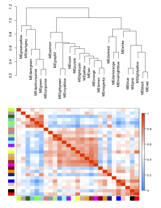
The top part of this plot represents the eigengene dendrogram and the lower part of this plot represents the eigengene adjacency heatmap.

3.6 Find the relationships between modules and traits

模块与性状之间的关系

#Plot the relationships between modules and traits
design = model.matrix(~0+ datTraits$subtype)
colnames(design) = levels(datTraits$subtype)
moduleColors = labels2colors(net$colors)
nGenes = ncol(datExpr)
nSamples = nrow(datExpr)
# Recalculate MEs with color labels
MEs0 = moduleEigengenes(datExpr, moduleColors)$eigengenes
MEs = orderMEs(MEs0)
moduleTraitCor = cor(MEs, design, use = "p")
moduleTraitPvalue = corPvalueStudent(moduleTraitCor, nSamples)

pdf(file="/Share2/home/lulab/xixiaochen/Share/xixiaochen/project/training/module_trait_relationship.pdf",width=9, height=10)
#Display the correlations and their p-values
textMatrix = paste(signif(moduleTraitCor, 2), "\n(",
                   signif(moduleTraitPvalue, 1), ")", sep = "")
dim(textMatrix) = dim(moduleTraitCor)
par(mar = c(6, 8.5, 3, 3))
#Display the correlation values within a heatmap plot
labeledHeatmap(Matrix = moduleTraitCor,
               xLabels = colnames(design),
               yLabels = names(MEs),
               ySymbols = names(MEs),
               colorLabels = FALSE,
               colors = blueWhiteRed(50),
               textMatrix = textMatrix,
               setStdMargins = FALSE,
               cex.text = 0.6,
               zlim = c(-1,1),
               main = paste("Module-trait relationships"))
dev.off()

通过模块与各种表型的相关系数，可以很清楚的挑选自己感兴趣的模块进行下游分析了。这个图就是把moduleTraitCor这个矩阵给用热图可视化一下。

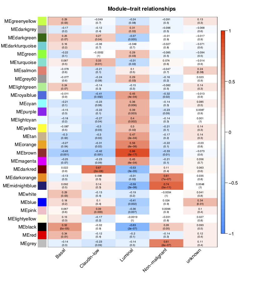
从上图已经可以看到跟乳腺癌分类相关的基因模块了，包括”Basal” “Claudin-low” “Luminal” “Non-malignant” “unknown” 这5类所对应的不同模块的基因列表。可以看到每一种乳腺癌都有跟它强烈相关的模块，可以作为它的表达signature，模块里面的基因可以拿去做下游分析。我们看到Luminal表型跟棕色的模块相关性高达0.86，而且极其显著的相关，所以值得我们挖掘，这个模块里面的基因是什么，为什么如此的相关呢？

3.7 Select specific module

We choose the “brown” module in trait “Luminal” for further analyses.

3.7.1 Intramodular connectivity, module membership, and screening for intramodular hub genes

#Intramodular connectivity, module membership, and screening for intramodular hub genes
#Intramodular connectivity
connet=abs(cor(datExpr,use="p"))^6
Alldegrees1=intramodularConnectivity(connet, moduleColors)

#Relationship between gene significance and intramodular connectivity
which.module="brown"
Luminal= as.data.frame(design[,3])
names(Luminal) = "Luminal"
GS1 = as.numeric(cor(datExpr, Luminal, use = "p"))
GeneSignificance=abs(GS1)

#Generalizing intramodular connectivity for all genes on the array
datKME=signedKME(datExpr, MEs, outputColumnName="MM.")
#Display the first few rows of the data frame

#Finding genes with high gene significance and high intramodular connectivity in specific modules
#abs(GS1)>.8 #adjust parameter based on actual situations
#abs(datKME$MM.black)>.8 #at least larger than 0.8
FilterGenes= abs(GS1)>0.8 & abs(datKME$MM.brown)>0.8
table(FilterGenes)
#FilterGenes
#FALSE  TRUE 
#4997     3
#find 3 hub genes
hubgenes <- rownames(datKME)[FilterGenes]
hubgenes
#[1] "ENSG00000124664" "ENSG00000129514" "ENSG00000143578"

3.7.2 Export the network

#Export the network
#Recalculate topological overlap
TOM = TOMsimilarityFromExpr(datExpr, power = 6) 
# Select module
module = "brown"
# Select module probes
probes = colnames(datExpr)
inModule = (moduleColors==module)
modProbes = probes[inModule] 
# Select the corresponding Topological Overlap
modTOM = TOM[inModule, inModule]
dimnames(modTOM) = list(modProbes, modProbes)

#Export the network into edge and node list files Cytoscape can read
#default threshold = 0.5, we could adjust parameter based on actual situations or in Cytoscape
cyt = exportNetworkToCytoscape(modTOM,
    edgeFile = paste("CytoscapeInput-edges-", paste(module, collapse="-"), ".txt", sep=""),
    nodeFile = paste("CytoscapeInput-nodes-", paste(module, collapse="-"), ".txt", sep=""),
    weighted = TRUE,
    threshold = 0.02,
    nodeNames = modProbes, 
    nodeAttr = moduleColors[inModule])

#Screen the top genes
nTop = 10
IMConn = softConnectivity(datExpr[, modProbes])
top = (rank(-IMConn) <= nTop)
filter <- modTOM[top, top]

cyt = exportNetworkToCytoscape(filter,
    edgeFile = paste("CytoscapeInput-edges-filter-", paste(module, collapse="-"), ".txt", sep=""),
    nodeFile = paste("CytoscapeInput-nodes-filter-", paste(module, collapse="-"), ".txt", sep=""),
    weighted = TRUE,
    threshold = 0.02,
    nodeNames = rownames(filter), 
    nodeAttr = moduleColors[inModule][1:nTop])

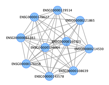
This plot is visualized by Cytoscape.

The output files look like:

#Bash Shell command:
head CytoscapeInput-edges-filter-brown.txt
#fromNode    toNode    weight    direction    fromAltName    toAltName
#ENSG00000108639    ENSG00000124664    0.0597956525080059    undirected    NA    NA
#ENSG00000108639    ENSG00000214530    0.0618251730361535    undirected    NA    NA
#ENSG00000108639    ENSG00000129514    0.0339542369643292    undirected    NA    NA
#ENSG00000108639    ENSG00000065361    0.0360849044869507    undirected    NA    NA

##Bash Shell command:
head CytoscapeInput-nodes-filter-brown.txt
#nodeName    altName    nodeAttr.nodesPresent...
#ENSG00000108639    NA    brown
#ENSG00000124664    NA    brown
#ENSG00000214530    NA    brown
#ENSG00000129514    NA    brown

3.7.3 Extract gene IDs in specific module

#Extract gene IDs in specific module
#Select module
module = "brown"
#Select module probes (gene ID)
probes = colnames(datExpr)
inModule = (moduleColors == module)
modProbes = probes[inModule]
write.table(modProbes,file="/Share2/home/lulab/xixiaochen/Share/xixiaochen/project/training/geneID_brown.txt",sep="\t",quote=F,row.names=F,col.names=F)

The output file looks like:

head geneID_brown.txt
#ENSG00000170421
#ENSG00000111057
#ENSG00000092841
#ENSG00000169710
#ENSG00000189334

We could use the gene ID list for GO/KEGG analysis.

4 Appendix：functional annotation of lncRNA

4.1 GO/KEGG analysis of the module which interested lncRNAs are involved in.

在WGCNA得到模块之后，通过fisher exact test分析感兴趣的lncRNA(例如：上调或者下调)是否在这些模块中显著富集，挑选出显著富集的模块中的protein coding genes做功能分析。

4.2 Construct the lncRNA-mRNA co-expression network, functional analysis of mRNAs which are co-expressed with these interested lncRNAs.

Library packages and load the input data

library(multtest)
lnc_mRNA_dataExpr2 <- readRDS(file="/Share2/home/lulab/xixiaochen/Share/xixiaochen/project/training/lnc_mRNA_dataExpr2.rds")

The input file looks like:

dim(lnc_mRNA_dataExpr2)
#[1]     6 2000
#The input data contains 6 samples, 2000 genes (1500 protein coding genes, 500 lncRNAs). 
lnc_mRNA_dataExpr2[1:4,1:4]
#         ENSMUSG00000000031.16 ENSMUSG00000006462.6 ENSMUSG00000006638.14 ENSMUSG00000010492.10
#Ctrl1Hip             0.0000000             0.249761              0.186874               0.120363
#Ctrl2Hip             0.0510846             0.157029              0.221414               0.272098
#Ctrl3Hip             0.0504136             0.168071              0.373061               0.134684
#RF1Hip               0.0000000             0.166485              0.250347               0.492554
####Each row represents a sample, each column represents a gene

Calculate the pearson correlation between every two genes.

#Calculate the pearson correlation
Pcc = cor(lnc_mRNA_dataExpr2, method = "pearson")

#Calculate the p-values of the pearson correlation
Pcc_pvalue = corPvalueFisher(Pcc, 6, twoSided = TRUE)

dim(Pcc)
#[1] 2000 2000
Pcc[1:4,1:4]
#                      ENSMUSG00000000031.16 ENSMUSG00000006462.6 ENSMUSG00000006638.14 ENSMUSG00000010492.10
#ENSMUSG00000000031.16            1.00000000            0.1619654            0.09256716            -0.4244842
#ENSMUSG00000006462.6             0.16196545            1.0000000           -0.50330176            -0.5484968
#ENSMUSG00000006638.14            0.09256716           -0.5033018            1.00000000            -0.2397083
#ENSMUSG00000010492.10           -0.42448423           -0.5484968           -0.23970829             1.0000000

dim(Pcc_pvalue)
#[1] 2000 2000
Pcc_pvalue[1:4,1:4]
#                      ENSMUSG00000000031.16 ENSMUSG00000006462.6 ENSMUSG00000006638.14 ENSMUSG00000010492.10
#ENSMUSG00000000031.16             0.0000000            0.7771578             0.8722577             0.4325254
#ENSMUSG00000006462.6              0.7771578            0.0000000             0.3375244             0.2858186
#ENSMUSG00000006638.14             0.8722577            0.3375244             0.0000000             0.6719851
#ENSMUSG00000010492.10             0.4325254            0.2858186             0.6719851             0.0000000

write.table(Pcc, file ="/Share2/home/lulab/xixiaochen/training_share2/co_expression/pcc.txt", quote = F, row.names = F, sep="\t")
write.table(Pcc_pvalue, file ="/Share2/home/lulab/xixiaochen/training_share2/co_expression/pcc_pvalue.txt", quote = F,row.names = F, sep="\t")

#Get the row and column names
pcc_pvalue_colnames=colnames(Pcc_pvalue)
pcc_pvalue_rownames=rownames(Pcc_pvalue)

write.table(pcc_pvalue_colnames, file ="/Share2/home/lulab/xixiaochen/training_share2/co_expression/Pcc_pvalue_colnames.txt", quote = F, row.names = F, sep="\t")
write.table(pcc_pvalue_rownames, file ="/Share2/home/lulab/xixiaochen/training_share2/co_expression/Pcc_pvalue_rownames.txt", quote = F, row.names = F, sep="\t")

#Bash Shell command:
#Extract the "protein coding gene & lncRNA" gene-gene pairs
sed -n '502,2001p' pcc_pvalue.txt | cut -f 1-500 > lnc_coding_pvalue.txt
sed -n '502,2001p' pcc.txt | cut -f 1-500 > lnc_coding_pcc.txt

#use the multtest package
raw_pvalue = read.table("/Share2/home/lulab/xixiaochen/training_share2/co_expression/lnc_coding_pvalue.txt", sep='\t', quote="", comment="")
#The input file looks like
dim(raw_pvalue)
#[1] 1500  500
raw_pvalue[1:4,1:4]
#           V1        V2        V3        V4
#1 0.4096710 0.396465705 0.2057436 0.80999264
#2 0.6188956 0.004920709 0.6733839 0.20778508
#3 0.5070725 0.931732205 0.7584698 0.66705000
#4 0.9983747 0.465891803 0.3436047 0.03568696
#2000 genes = 1500 protein coding genes, 500 lncRNAs
#Each row represents a protein-coding gene, each column represents a lncRNA.
#The row names are in the "Pcc_pvalue_rownames.txt" file, the column names are in the "Pcc_pvalue_colnames.txt".

#Calculate the adjusted p-values
setwd("/Share2/home/lulab/xixiaochen/training_share2/co_expression/adjp/")
#the multtest package: output=adjusted p-values from small to large order, index=original row and column information
for (i in seq(1,dim(raw_pvalue)[2])){
  ad=mt.rawp2adjp(raw_pvalue[,i], proc=c("Bonferroni"))
  adjp=ad$adjp[,2]
  order_index=ad$index
  re=matrix=cbind(adjp,order_index)
  out_file=paste(as.character(i),'txt',sep='.')
  write.table(re, file =out_file, quote = F, row.names = F,sep="\t")
}

In the previous step, we will get 500 files. In this step, process these file to get gene pairs with an adjusted P-value of 0.01 or less and with a Pcc value ranked in the top or bottom 0.05 percentile.

#Bash Shell command:
python get_gene_pairs.py
perl get_gene_pairs.pl adjp_cut.txt pcc_cut.txt gene_pairs.txt

the get_gene_pairs.py contains:

import pandas as pd
import numpy as np
import os
fold_path='/Share2/home/lulab/xixiaochen/training_share2/co_expression/adjp/'
file_li=os.listdir(fold_path)
adjp_fi_li=[]
for i in range(len(file_li)):
    adjp_pre_li=[]
    file_name=str(i+1)+'.txt'
    file_path=fold_path+file_name
    #print file_path
    data=pd.read_csv(file_path,sep='\t')
    data=data.set_index('order_index').sort_index()
    adjp=data['adjp']
    adjp_pre_li=list(adjp)
    adjp_fi_li.append(adjp_pre_li)
fi_adjp=pd.DataFrame(adjp_fi_li)
adjp_T=fi_adjp.T
comp_adjp=adjp_T[adjp_T<0.01]
#add gene names, each row represents a protein-coding gene, each column represents a lncRNA
col_file='/Share2/home/lulab/xixiaochen/training_share2/co_expression/Pcc_pvalue_colnames.txt'
row_file='/Share2/home/lulab/xixiaochen/training_share2/co_expression/Pcc_pvalue_rownames.txt'
col=pd.read_csv(col_file)
colnames=list(col['x'])[:500]
row=pd.read_csv(row_file)
rownames=list(row['x'])[500:]
def com_get_pair(df):
    df.columns=colnames
    df.index=rownames
    a=[]
    for i in range(df.index.size):
        for j in range(df.columns.size):
            b=[]
            if not np.isnan(df.iloc[i][j]):
                #add the row names
                b.append(df.iloc[i].name)
                #add the column names
                b.append(df.iloc[:,j].name)
                #add value
                b.append(df.iloc[i][j])
                a.append(b)
    df_df=pd.DataFrame(a)
    df_df.columns=['coding genes','lncRNA','Pcc']
    return df_df
#filter Pcc in top 5%
pcc_file='/Share2/home/lulab/xixiaochen/training_share2/co_expression/lnc_coding_pcc.txt'
pcc=pd.read_csv(pcc_file,sep='\t',header=None)
#filter Pcc in bottom 5%
pcc=abs(pcc)
all_pcc=[]
for i in range(pcc.columns.size):
    all_pcc.extend(list(pcc.iloc[:,i]))
all_pcc_se=pd.Series(all_pcc)
cut_pcc=all_pcc_se.quantile(0.95)
pcc_cut=pcc[pcc>cut_pcc]
pcc_df=com_get_pair(pcc_cut)
adjp_df=com_get_pair(comp_adjp)
pcc_out_file='/Share2/home/lulab/xixiaochen/training_share2/co_expression/pcc_cut.txt'
pcc_df.to_csv(pcc_out_file,sep='\t',index=False)
adjp_out_file='/Share2/home/lulab/xixiaochen/training_share2/co_expression/adjp_cut.txt'
adjp_df.to_csv(adjp_out_file,sep='\t',index=False)

the get_gene_pairs.pl contains:

#! /usr/bin/perl
open I1, "<$ARGV[0]";
open I2, "<$ARGV[1]";
open OUT, ">$ARGV[2]";
my %list;
while(<I1>){
    chomp;
    @data0 = split/\t/,$_;
    if(/^coding(.*)/){}
    else{
        $list{$data0[0].$data0[1]} = $data0[2];
    }
}
while(<I2>){
    chomp;
    @data = split/\t/,$_;
    if(/^coding(.*)/){
        print OUT "mRNA\tlncRNA\tpcc\tadjp\n";
    }
    if(exists $list{$data[0].$data[1]}){
        $adjp = $list{$data[0].$data[1]};
        print OUT "$_\t$adjp\n";
    }
}        
close I1;
close I2;
close OUT;

In the “python get_gene_pairs.py” step, the input files include:

File name	Description
All files in the “~/adjp/” directory	The 5,196 files are the results for adjusted p-values
Pcc_pvalue_colnames.txt	Column names for the adjusted p-value matrix
Pcc_pvalue_rownames.txt	Row names for the adjusted p-value matrix
lnc_coding_pcc.txt	Pcc value matrix, each row represent a protein-coding gene, each column represent a lncRNA

Please make sure all the input files and the python script are in the same work directory.

The output files looks like:

#Bash Shell command:
head pcc_cut.txt
#coding genes            lncRNA                    Pcc
#ENSMUSG00000085431.7	ENSMUSG00000033015.16	1.0
#ENSMUSG00000085431.7	ENSMUSG00000037910.2	1.0
#ENSMUSG00000085431.7	ENSMUSG00000038152.4	0.898454912289789
#ENSMUSG00000085431.7	ENSMUSG00000039545.15	0.940380543474745
#ENSMUSG00000085431.7	ENSMUSG00000040657.3	1.0
#ENSMUSG00000085431.7	ENSMUSG00000041674.16	0.8245987116435991
#Each row show a protein-coding gene & lncRNA gene-gene pair, and their Pcc value.

head adjp_cut.txt
#coding genes            lncRNA                   Pcc
#ENSMUSG00000085431.7	ENSMUSG00000033015.16	0.0
#ENSMUSG00000085431.7	ENSMUSG00000037910.2	0.0
#ENSMUSG00000085431.7	ENSMUSG00000040657.3	0.0
#ENSMUSG00000085431.7	ENSMUSG00000055159.7	0.0
#ENSMUSG00000085431.7	ENSMUSG00000073144.4	0.0
#ENSMUSG00000085431.7	ENSMUSG00000073652.10	0.0048784147212109
#Each row show a protein-coding gene & lncRNA gene-gene pair, and their adjusted p-value.

In the “perl get_gene_pairs.pl adjp_cut.txt pcc_cut.txt gene_pairs.txt” step, the input files include:

Please make sure all the input files and the perl script are in the same work directory.

File name	Description
pcc_cut.txt	Pcc values of the “protein-coding gene & lncRNA” gene-gene pairs
adjp_cut.txt	Adjusted p-value of the “protein-coding gene & lncRNA” gene-gene pairs

the output file looks like:

head gene_pairs.txt 
#mRNA                     lncRNA                  pcc               adjp
#ENSMUSG00000085431.7	ENSMUSG00000033015.16	1.0	0.0
#ENSMUSG00000085431.7	ENSMUSG00000037910.2	1.0	0.0
#ENSMUSG00000085431.7	ENSMUSG00000040657.3	1.0	0.0
#ENSMUSG00000085431.7	ENSMUSG00000055159.7	1.0	0.0
#ENSMUSG00000085431.7	ENSMUSG00000073144.4	1.0	0.0
#ENSMUSG00000085431.7	ENSMUSG00000073652.10	0.9907736676388159	0.0048784147212109
#Each row show a protein-coding gene & lncRNA gene-gene pair, and their Pcc value, adjusted p-value.

We could extract the mRNA gene set for GO/KEGG analysis.

5 Homework

Inputdata:

/Share2/home/lulab/xixiaochen/training_share2/co_expression/homework_FemaleLiver-01-dataInput.RData
134 samples, 3600 genes; each row represents a sample, each column represents a gene.

Please try to construct an automatic network and detect module (Choosing the soft-thresholding power, One-step network construction and module detection). Please plot two figures: 1.Analysis of network topology(Scale independence, Mean connectivity) for various soft-thresholding powers, 2.The dendrogram and the module colors underneath.

6.Reference

https://github.com/jmzeng1314/my_WGCNA

https://horvath.genetics.ucla.edu/html/CoexpressionNetwork/Rpackages/WGCNA/Tutorials/index.html

example

training_class

Co-expression

Co-expression

1.Pipeline

2.Data structure

2.1.Getting software & data

2.2.Input data

2.3 Output data

3.Running steps

WGCNA分析

基本概念

基本原理

3.0 Install packages

3.1 Library the WGCNA package

3.2 Pick the soft thresholding power

3.3 One-step network construction and module detection

3.4 Module visualization

3.5 Quantify module similarity by eigengene correlation

3.6 Find the relationships between modules and traits

3.7 Select specific module

3.7.1 Intramodular connectivity, module membership, and screening for intramodular hub genes

3.7.2 Export the network

3.7.3 Extract gene IDs in specific module

4 Appendix：functional annotation of lncRNA

4.1 GO/KEGG analysis of the module which interested lncRNAs are involved in.

4.2 Construct the lncRNA-mRNA co-expression network, functional analysis of mRNAs which are co-expressed with these interested lncRNAs.

5 Homework

6.Reference